Daily Insights on Scientific Python

Solving both common and complex problems using Numpy, Sympy, SciPy, and Matplotlib.

The Challenge

Consider the following code snippet where we establish a one-dimensional equidistant grid, denoted as x:

One of NumPy's strengths is its ability to apply functions seamlessly across arrays. For instance, we can compute the sine values over this grid as follows:

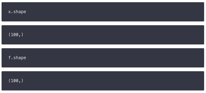
Both x and f are one-dimensional arrays, each containing 100 elements as expected:

This process is quite straightforward. However, what if we need to work in multiple dimensions? How do we utilize a two-dimensional grid along the x and y axes? Specifically, how can we compute the function:

The Solution

To begin, we define our one-dimensional coordinate values just as we did in the single-dimensional scenario.

While you could technically write:

This approach would only yield a one-dimensional array. NumPy cannot infer that these one-dimensional arrays represent coordinate values or that the two axes intersect perpendicularly. This is where mesh grids become essential.

In a two-dimensional environment, a mesh grid consists of two arrays: one for the x-coordinates and another for the y-coordinates. These arrays are generated by combining all possible x and y values within designated ranges. Each combination corresponds to a specific point on the grid, resulting in a rectangular layout where each point possesses unique x and y coordinates.

For example, if we want to create a mesh grid with x values ranging from 0 to 2 and y values from 0 to 3, the resulting mesh grid would produce two-dimensional X and Y arrays as follows:

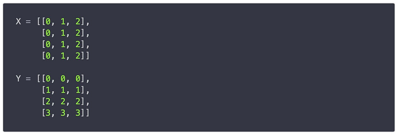
I typically use lowercase letters for the 1-D coordinate arrays, such as x, and uppercase letters for the meshed grid versions, like X. Here, each element in the X array corresponds to the x-coordinate of a point on the two-dimensional grid, while each element in the Y array corresponds to the y-coordinate.

The meshgrid function in NumPy streamlines the creation of mesh grids. It takes one or more one-dimensional arrays representing coordinates along each dimension and returns a set of arrays that form the mesh grid.

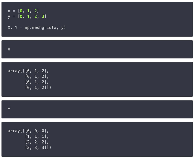
The resulting output arrays share the same shape, which corresponds to the shape of the input arrays when combined:

With the mesh grid established, we can now compute our function over the two-dimensional grid:

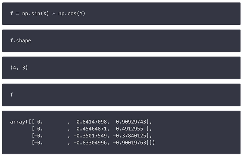
Note that the first axis (axis 0) has a length of 4, while the second axis (axis 1) has a length of 3. Comparing this to the one-dimensional coordinate arrays x and y, you can see that meshgrid has assigned all values to axis 0 of the resulting mesh grid and the corresponding values to axis 1.

To access the function value at the point (x[1], y[3]), we would use the syntax:

Depending on the context, this may feel somewhat counterintuitive because we often visualize the x-axis as the first axis and the y-axis as the second. However, this ordering is standard in image processing, where the first axis is viewed as vertical and the second as horizontal.

To align with the more familiar mathematical representation, we can modify the behavior of meshgrid by using the indexing='ij' option:

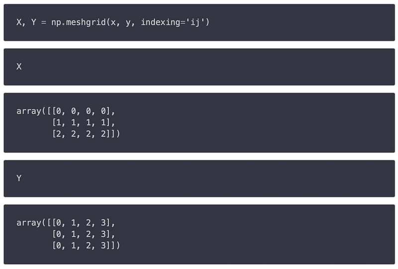
Now, the use of our grid becomes more intuitive for our needs. We redefine:

And we can easily retrieve the function value for the second point (index 1) on the x-axis and the fourth point (index 3) on the y-axis by calling:

Conclusion

The meshgrid function in NumPy is a valuable tool for generating coordinate systems in multiple dimensions. It enables the creation of meshgrid arrays that represent grid points, each with distinct coordinates. By inputting one or more one-dimensional arrays for the coordinates along each dimension, meshgrid simplifies the process of constructing these grids.

The default indexing option generates output arrays where the x-coordinates match the shape of the y-value input array, while the y-coordinates correspond with the shape of the x-value input array. This convention is particularly useful for image processing applications.

Alternatively, using the ‘ij’ indexing option allows for output arrays where the x-coordinates align with the shape of the x-value input array, and the y-coordinates match the shape of the y-value input array. This indexing style may be more suitable in various mathematical contexts.

Exploring NumPy's Meshgrid in Action

To further enhance your understanding of mesh grids in NumPy, watch the following videos:

The first video, titled "NumPy Meshgrid - Understanding np.meshgrid() [Simple Guide]," provides an accessible overview of the meshgrid function and its applications.

The second video, "Meshgrid Explained Python | 3D Plotting | Matplotlib and NumPy | Programming," delves deeper into mesh grids, showcasing their use in 3D plotting and programming contexts.